Attention (machine learning)

Given a sequence of tokens ${\displaystyle t_{i}}$ labeled by the index ${\displaystyle i}$, a neural network computes a soft weight ${\displaystyle w_{i}}$ for each ${\displaystyle t_{i}}$ with the property that ${\displaystyle w_{i}}$ is non-negative and ${\textstyle \sum _{i}w_{i}=1}$. Each ${\displaystyle t_{i}}$ is assigned a value vector ${\displaystyle v_{i}}$ which is computed from the word embedding of the ${\displaystyle i}$th token. The weighted average ${\textstyle \sum _{i}w_{i}v_{i}}$ is the output of the attention mechanism.

The query-key mechanism computes the soft weights. From the word embedding of each token, it computes its corresponding query vector ${\displaystyle q_{i}}$ and key vector ${\displaystyle k_{i}}$. The weights are obtained by taking the softmax function of the dot product ${\displaystyle q_{i}k_{j}}$ where ${\displaystyle i}$ represents the current token and ${\displaystyle j}$ represents the token that's being attended to.

In some architectures, there are multiple "heads" of attention (termed 'multi-head attention'), each operating independently with their own queries, keys, and values.

To build a machine that translates English to French, one takes the basic Encoder-Decoder and grafts an attention unit to it (diagram below). In the simplest case, the attention unit consists of dot products of the recurrent encoder states and does not need training. In practice, the attention unit consists of 3 fully-connected neural network layers called query-key-value that need to be trained. See the Variants section below.

Encoder-decoder with attention. The left part (black lines) is the encoder-decoder, the middle part (orange lines) is the attention unit, and the right part (in grey & colors) is the computed data. Grey regions in H matrix and w vector are zero values. Numerical subscripts indicate vector sizes while lettered subscripts i and i − 1 indicate time steps.

Viewed as a matrix, the attention weights show how the network adjusts its focus according to context.

This view of the attention weights addresses the "explainability" problem that neural networks are criticized for. Networks that perform verbatim translation without regard to word order would have a diagonally dominant matrix if they were analyzable in these terms. The off-diagonal dominance shows that the attention mechanism is more nuanced. On the first pass through the decoder, 94% of the attention weight is on the first English word "I", so the network offers the word "je". On the second pass of the decoder, 88% of the attention weight is on the third English word "you", so it offers "t'". On the last pass, 95% of the attention weight is on the second English word "love", so it offers "aime".

There are many variants of attention that implements soft weights, including (a) Bahdanau Attention,[8] also referred to as additive attention, and (b) Luong Attention [9] which is known as multiplicative attention, built on top of additive attention, and (c) self-attention introduced in transformers. For convolutional neural networks, the attention mechanisms can also be distinguished by the dimension on which they operate, namely: spatial attention,[10] channel attention,[11] or combinations of both.[12][13]

These variants recombine the encoder-side inputs to redistribute those effects to each target output. Often, a correlation-style matrix of dot products provides the re-weighting coefficients (see legend).

1. encoder-decoder dot product	2. encoder-decoder QKV	3. encoder-only dot product	4. encoder-only QKV	5. Pytorch tutorial
Both encoder & decoder are needed to calculate attention.[9]	Both encoder & decoder are needed to calculate attention.[14]	Decoder is not used to calculate attention. With only 1 input into corr, W is an auto-correlation of dot products. wij = xi xj[15]	Decoder is not used to calculate attention.[16]	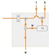A fully-connected layer is used to calculate attention instead of dot product correlation.[17]

• Transformer (machine learning model) § Scaled dot-product attention
• Perceiver § Components for query-key-value (QKV) attention

• Dan Jurafsky and James H. Martin (2022) Speech and Language Processing (3rd ed. draft, January 2022), ch. 10.4 Attention and ch. 9.7 Self-Attention Networks: Transformers
• Alex Graves (4 May 2020), Attention and Memory in Deep Learning (video lecture), DeepMind / UCL, via YouTube
• Rasa Algorithm Whiteboard - Attention via YouTube

References

- Yann Lecun (2020). Deep Learning course at NYU, Spring 2020, video lecture Week 6. Event occurs at 53:00. Retrieved 2022-03-08.
- Graves, Alex; Wayne, Greg; Reynolds, Malcolm; Harley, Tim; Danihelka, Ivo; Grabska-Barwińska, Agnieszka; Colmenarejo, Sergio Gómez; Grefenstette, Edward; Ramalho, Tiago; Agapiou, John; Badia, Adrià Puigdomènech; Hermann, Karl Moritz; Zwols, Yori; Ostrovski, Georg; Cain, Adam; King, Helen; Summerfield, Christopher; Blunsom, Phil; Kavukcuoglu, Koray; Hassabis, Demis (2016-10-12). "Hybrid computing using a neural network with dynamic external memory". Nature. 538 (7626): 471–476. Bibcode:2016Natur.538..471G. doi:10.1038/nature20101. ISSN 1476-4687. PMID 27732574. S2CID 205251479.
- Vaswani, Ashish; Shazeer, Noam; Parmar, Niki; Uszkoreit, Jakob; Jones, Llion; Gomez, Aidan N.; Kaiser, Lukasz; Polosukhin, Illia (2017-12-05). "Attention Is All You Need". arXiv:1706.03762 [cs.CL].
- Ramachandran, Prajit; Parmar, Niki; Vaswani, Ashish; Bello, Irwan; Levskaya, Anselm; Shlens, Jonathon (2019-06-13). "Stand-Alone Self-Attention in Vision Models". arXiv:1906.05909 [cs.CV].
- Jaegle, Andrew; Gimeno, Felix; Brock, Andrew; Zisserman, Andrew; Vinyals, Oriol; Carreira, Joao (2021-06-22). "Perceiver: General Perception with Iterative Attention". arXiv:2103.03206 [cs.CV].
- Ray, Tiernan. "Google's Supermodel: DeepMind Perceiver is a step on the road to an AI machine that could process anything and everything". ZDNet. Retrieved 2021-08-19.
- "Pytorch.org seq2seq tutorial". Retrieved December 2, 2021.
- Bahdanau, Dzmitry (2016-05-19). "Neural Machine Translation by Jointly Learning to Align and Translate". arXiv:1409.0473 [cs.CL].
- Luong, Minh-Thang (2015-09-20). "Effective Approaches to Attention-based Neural Machine Translation". arXiv:1508.04025v5 [cs.CL].
- Zhu, Xizhou; Cheng, Dazhi; Zhang, Zheng; Lin, Stephen; Dai, Jifeng (2019). "An Empirical Study of Spatial Attention Mechanisms in Deep Networks". 2019 IEEE/CVF International Conference on Computer Vision (ICCV): 6687–6696. arXiv:1904.05873. doi:10.1109/ICCV.2019.00679. ISBN 978-1-7281-4803-8. S2CID 118673006.
- Hu, Jie; Shen, Li; Sun, Gang (2018). "Squeeze-and-Excitation Networks". IEEE/CVF Conference on Computer Vision and Pattern Recognition: 7132–7141. arXiv:1709.01507. doi:10.1109/CVPR.2018.00745. ISBN 978-1-5386-6420-9. S2CID 206597034.
- Woo, Sanghyun; Park, Jongchan; Lee, Joon-Young; Kweon, In So (2018-07-18). "CBAM: Convolutional Block Attention Module". arXiv:1807.06521 [cs.CV].
- Georgescu, Mariana-Iuliana; Ionescu, Radu Tudor; Miron, Andreea-Iuliana; Savencu, Olivian; Ristea, Nicolae-Catalin; Verga, Nicolae; Khan, Fahad Shahbaz (2022-10-12). "Multimodal Multi-Head Convolutional Attention with Various Kernel Sizes for Medical Image Super-Resolution". arXiv:2204.04218 [eess.IV].
- Neil Rhodes (2021). CS 152 NN—27: Attention: Keys, Queries, & Values. Event occurs at 06:30. Retrieved 2021-12-22.
- Alfredo Canziani & Yann Lecun (2021). NYU Deep Learning course, Spring 2020. Event occurs at 05:30. Retrieved 2021-12-22.
- Alfredo Canziani & Yann Lecun (2021). NYU Deep Learning course, Spring 2020. Event occurs at 20:15. Retrieved 2021-12-22.
- Robertson, Sean. "NLP From Scratch: Translation With a Sequence To Sequence Network and Attention". pytorch.org. Retrieved 2021-12-22.
External links